How-To
Researchers Discover New Technique for Training Huge Neural Networks
It can train huge neural networks in a fraction of the time and cost required for standard training techniques.
- By Pure AI Editors
- 04/04/2022
Machine learning researchers have demonstrated a new technique that can train huge neural networks in a fraction of the time and cost required for standard training techniques. Briefly, it's possible to start with a carefully designed small version of the huge network, find optimal training parameters for it, and then apply those parameters when training the goal huge network. Designing the small network is called "maximal update parameterization." Using the optimal training parameters on a huge network is called "mu transfer."
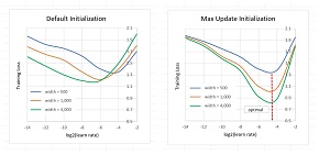 [Click on image for larger view.] Figure 1: Maximal Update Parameter Networks Share Optimal Learning Rate
The research paper that describes the new training technique is "Tuning Large Neural Networks via Zero-Shot Hyperparameter Transfer" by G. Yang, E. Hu, I. Babuschkin, S. Sidor, D. Farhi, J. Pachocki, X. Liu, W. Chen, and J. Gao. The paper can be found in several locations on the internet.
Note: The research ideas described here are complex and subtle. Several simplifications have been made in order to shorten and clarify the explanations.
A Concrete Example
A concrete example makes the ideas of mu transfer training easier to grasp. Suppose you want to train a natural language model/network that has 1,000,000,000,000 weights which must be learned. Each weight is a numeric constant, often between -10.0 and +10.0. Training the model is the process of finding good values for the weights so that the model predicts with high accuracy.
In order to train the huge model, you must specify how to initialize the weights (for example, using random values between -1.0 and +1.0) and you must specify training parameters such as the learning rate (how quickly weights change during training), the batch size (how many training items to process at a time), the learning rate schedule (how to gradually decrease the learning rate during training), and so on.
There are essentially an infinite number of combinations of weight initializations and training parameters, and examining each combination takes a lot of time (possibly days) and money (often tens or hundreds of thousands of dollars) per attempt. It's simply not feasible to try many different training parameter values, and so you must use your best guess, train the huge model, and hope for a good result.
In the newly discovered training technique, you create a relatively small version of the model with, say, 1,000,000 weights. With a neural network of this size, it is feasible to use one of several techniques to experiment and find the optimal or near-optimal set of training parameters. For example, after running 100 experiments you might find, "Optimal training uses a learning rate of 0.014, with a batch size of 512, and an exponential decay learning rate schedule with gamma of 0.9985."
If the small 1,000,000-weight network has been constructed carefully, the optimal training parameters for the small network are also optimal for an expanded version of the network that has 1,000,000,000,000 weights. You can train the huge model just once using the optimal training parameters that were discovered for the smaller network. This will still be expensive, but you have confidence you've used the best, or near-best, training parameters.
To summarize, if you want to train a huge neural network model, you first create a smaller version of the network using specific network architecture parameters. This is called "maximal update parametrization". You train the small network several times and find good training parameters such as the learning rate. The good training parameters can be used to train the huge network one time. This is called "mu transfer."
Creating a Small Network
A standard neural network architecture has input nodes, several layers of hidden nodes where most of the computational work is done, and output nodes. The number of input nodes and the number of output nodes are determined by the problem being solved. For example, in MNIST image classification, the goal is to determine a handwritten digit from "0" to "9" where each image has 28 by 28 = 784 pixels. Therefore, a neural network model will have 784 input nodes and 10 output nodes. However, the number of hidden layers, and the number of nodes in each hidden layer are hyperparameters that must be determined by trial and error.
The number of hidden layers is usually called the depth of the network. The number of hidden nodes in each layer is called the width of the network. In the mu transfer training technique, the small preliminary neural network has the same depth (number hidden layers) but smaller width (number of nodes in each hidden layer). The diagram in Figure 2 shows a simplified network with depth = 3 and width = 4. Each line connecting a pair of nodes represents a weight value that must be learned during training. As the depth and width of a network increase, the number of weights that must be learned increases very quickly (specifically, quadratic increase).
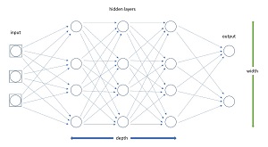 [Click on image for larger view.] Figure 2: Neural Network Width and Depth
Modern neural networks for difficult problems such as natural language processing don't use simple network architectures, but the principles are the same. The BERT (Bidirectional Encoder Representations from Transformers) language model uses what is called transformer architecture and has 350 million weights. The GPT-3 (Generative Pretrained Transformer version 3) model also uses a transformer architecture; it has 6.7 billion weights.
In the early days of large neural networks, there was an emphasis on increasing the depth of neural networks. More recently the emphasis is on increasing the width. This emphasis on network width is based on the surprising discovery that over-parameterization (using a much larger number of hidden nodes than necessary) leads to improved prediction models.
Mu Transfer
The two graphs in Figure 1 illustrate the key ideas behind the mu transfer training technique. The graph on the left represents a hypothetical neural network with a fixed depth and varying widths of 500, 1000, and 4000 nodes. The network is initialized using standard default parameters such as Kaiming weight initialization. As the learning rate varies (values on the left-right x-axis), the model loss varies. Smaller values of loss are better. The best learning rate is the lowest point on each graph and is different for each network width.
The graph on the right represents the same hypothetical network, but initialized using the maximal update parameterization technique. The optimal learning rate, indicated by the dashed red line, is the same for all three widths. In other words, it's possible to experiment and find the best learning rate for the small network, and then use it on a larger, scaled-up version of the network.
The research paper reports the results of several experiments that show the effectiveness of the maximal update parameter plus mu transfer training technique. For example, in an experiment with the BERT language model (350 million parameters), starting with a relatively small network with 13 million parameters, the mu transfer technique outperformed published results with a total tuning cost equivalent to pretraining once. And for the GPT-3 model (6.7 billion parameters), starting with a relatively small network with 40 million parameters, the mu transfer technique outperformed published results with tuning cost only 7 percent of total pretraining cost.
From Theory to Practice
The Hyperparameter Transfer research paper is 47 pages long and is mathematically intimidating. Furthermore, the research is based on several previous papers with hundreds of additional pages. Implementing the maximal update parameterization for the small network is tricky, but the researchers have created a PyTorch implementation that is available at https:www/github.com/microsoft/mup.
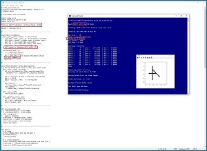 [Click on image for larger view.] Figure 3: Maximal Update Parametrization Library Code Demo in Action
The screenshot in Figure 3 shows a partial example of using the PyTorch implementation of maximal update parameter code. The screenshot shows that training a simple neural network using maximal update parameterization is similar to training a regular neural network. The next steps, which are not shown, would be to find optimal training parameters and then train a scaled-up large version of the small network.
Wrapping Up
The Pure AI editors contacted Greg Yang from Microsoft Research, one of the lead researchers on the mu transfer project. Yang commented, "When we derived maximal update parameterization, I asked myself: OK theoretically this looks like the correct parametrization, but how would this correctness manifest in practice? Then I realized that correctness should imply that it uniquely enables hyperparameter transfer."
Yang added, "Then we tried it, and it really worked! I have to say I am still surprised it worked out so well, because typically, in deep learning at least, theoretical ideas will die by a thousand cuts before they make it to be practical."
The Pure AI editors spoke about mu transfer training with Dr. James McCaffrey, from Microsoft Research. McCaffrey commented, "The research papers on the mu transfer technique for training huge neural networks are theoretically interesting and impressive from a practical point of view."
McCaffrey added, "In my opinion, the ongoing research presented in the series of papers represents a significant advance in understanding how to train massive neural networks. This is especially important for natural language processing scenarios."