How-To
Researchers Explore Intelligent Sampling of Huge ML Datasets to Reduce Costs and Maintain Model Fairness
Also, less CO2 is emitted, which is a good thing because one researcher said: "The current approach for building ML models is not sustainable and we will hit a ceiling soon, if not already."
- By Pure AI Editors
- 05/03/2021
Researchers at Microsoft have devised a new technique to select an intelligent sample from a huge file of machine learning training data. The technique is called loss-proportional sampling. Briefly, a preliminary, crude prediction model is created using all source data, then loss (prediction error) information from the crude model is used to select a sample that is superior to a randomly selected sample.
The researchers demonstrated that using an intelligent sample of training data can generate prediction models that are fair. Additionally, the smaller size of the sample data enables quicker model training, which reduces the electrical energy required to train, which in turn reduces the CO2 emissions generated while training the model.
Loss-Proportional Sampling
The ideas are best explained by an artificial example. Suppose you want to create a sophisticated machine learning model that predicts the credit worthiness of a loan application, 0 = reject application, 1 = approve application. You have an enormous file of training data -- perhaps billions of historical data items. Each data item has predictor variables such as applicant age, sex, race, income, debt, savings and so on, and a class label indicating if the loan was repaid, 0 = failed to repay, 1 = successfully repaid loan.
Suppose that training your prediction model using the entire source dataset is not feasible for some reason, and so you must select a sample of the source data. If you take a simple random sample from the huge source data, the sample will likely miss relatively rare data items, such as applicants that have minority race or applicants who are very old. After you train your loan application model, the prediction accuracy for rare-feature applications will likely be poor because the model didn't see enough of such data items during training.
Before continuing with the example, you need to understand or recall how a binary classification model works. A typical binary prediction model accepts input predictor values such as age, sex and so on and emits a single value between 0.0 and 1.0 called a pseudo-probability. A pseudo-probability value that is less than 0.5 indicates class 0 (reject application) and a pseudo-probability greater than 0.5 indicates class 1 (approve application).
To create an intelligent loss-proportional sample, you start by creating a crude binary classification model using the entire large source dataset. The most commonly used crude binary classification technique is called logistic regression. Using modern techniques, training a logistic regression model using an enormous data file is almost always feasible, unlike creating a more sophisticated model using a deep neural network.
After you have trained the crude model, you run all items in the large source dataset through the model. This will generate a loss (error) value for each source item, which is a measure of how far the prediction is from the actual class label. For example, the loss information might look like:
(large source dataset)
item  prediction  actual   loss   prob of selection
[0]    0.80         1      0.04   1.5 * 0.04 = 0.06
[1]    0.50         0      0.25   1.5 * 0.25 = 0.37
[2]    0.90         1      0.01   1.5 * 0.01 = 0.02
[3]    0.70         1      0.09   1.5 * 0.09 = 0.13
. . .
[N]    0.85         1      0.02   1.5 * 0.02 = 0.03
Here the loss value is the square of the difference between the prediction and the actual class label, but there are many other loss functions that can be used. In general, the loss values for data items that have rare features will be greater than the loss values for normal data items.
Next, you map the loss for each source data item to a probability. In the example above, each loss value is multiplied by a constant lambda = 1.5. Now, suppose you want a sample of data that is 10 percent of the size of the large source data. You iterate through the source dataset. For each item, you select it and add it to the sample with its associated probability. In the example above, item [0] would be selected with prob = 0.06 (likely not selected), then item [1] would be selected with prob = 0.37 (more likely) and so on. You repeat until the sample has the desired number of data items.
At this point you could now use the small sample dataset generated by loss-proportional selection to create a prediction model using a sophisticated classifier, such as a deep neural network. You can use the sample dataset directly, but the prediction results will not be the same as the results if you were somehow able to train the sophisticated classifier on the entire source dataset. In situations where you want to get the nearly same prediction results using the sample dataset, you can compute an importance weight for each item. The importance weight is just 1 over the selection probability. For example:
(small sample dataset)
item  p(select)    w = importance weight
[0]    0.021        1 / 0.021 =  47.62
[1]    0.013        1 / 0.013 =  76.92
[2]    0.018        1 / 0.018 =  55.56
. . .
[n]    0.016        1 / 0.016 =  62.50
If you think about it you'll see that rare feature items have higher loss from the crude classifier and so they'll have a higher probability of being included in the sample. Normal class items are less likely to be selected, but that is balanced by the fact that there are many more of such items.
During training, you weight each item by multiplying the loss by its importance weight. Items that had a low probability of being selected into the sample will have higher importance weights. This balances the fact that low probability items are more rare in the sample than they were in the source dataset.
The example presented here is for binary classification. The loss-proportional sampling technique can also be used for multi-class classification (three or more classes to predict) and for regression problems (predicting a single numeric value).
Looking at the Details of the Technique
The simplified example presented here has taken several shortcuts and left out details to make the ideas easier to understand. The ideas are fully explained in a 2013 research paper titled "Loss-Proportional Subsampling for Subsequent ERM" by P. Mineiro and N. Karampatziakisis. The paper is available online in several locations. Note that the title of the paper uses the term "subsampling" rather than "sampling." This just means that a large source dataset is considered to be a sample from all possible problem data. Therefore, selecting from the source dataset gives a subsample.
The research paper focuses on generating a sample dataset where there are mathematical guarantees about the characteristics of the sample dataset relative to the large source dataset. They key equation presented in the paper is shown in Figure 1.
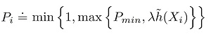 [Click on image for larger view.] Figure 1: Key Equation for Loss-Proportional Sampling
As is often the case, the key equation looks intimidating, but if you know what each symbol means the equation is quite simple. The Pi is the probability that data item Xi is selected from the source dataset for inclusion in the sample dataset. The equals sign with a dot means "is defined as." The Pmin value is a user-supplied minimum probability of selection. This prevents some data items from having no chance of being included in the sample dataset. The h(Xi) represents the loss value for data item Xi when it's fed to the preliminary crude prediction model. The Greek letter lambda is a user-supplied constant to map a loss value to a selection probability. The min{} notation essentially prevents a selection probability from being greater than 1.
The main challenge, when using loss-proportional sampling in practice, is balancing the values of Pmin and lambda relative to the magnitudes of loss values. If lambda is too large, most selection probabilities will be large, and data items that are at the beginning of the source dataset will be selected, filling the sample dataset, and none of the data items at the end of the source dataset will have a chance to be included. If Pmin is too large, it will overwhelm the computed selection probabilities.
Example: Toxic Comments
A Microsoft research and engineering team including Ziqi Ma, Paul Mineiro, KC Tung and James McCaffrey applied the loss-proportional sampling technique to the CivilComments benchmark dataset of online user comments. The dataset consists of 4.5 million comments that are labeled as normal (class 0) or toxic (class 1). An example of a toxic comment is, "Maybe you should learn to write a coherent sentence so we can understand WTF your point is." An example of a non-toxic comment is, "Black people should be judged based on their actions."
Many of the comments mention categories such as sex (male, female), race (black, white), religion (Christian, Muslim, other) and so on. As you'd expect, the distribution of comments with these categories is not even. The distribution of some of the categories is shown in the chart in Figure 2.
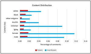 [Click on image for larger view.] Figure 2: Characteristics of the CivilComents Dataset
The point is that a model that predicts whether a comment is toxic or not will have relatively high accuracy on comments that include the most common categories, such as male and Christian, but the model will have lower prediction accuracy on comments with rare categories, such as black and "other" religions.
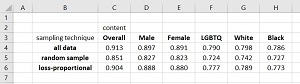
Partial results of the Microsoft experiments are shown in the table in Figure 3. Three machine learning prediction models were created. One model used all 4.5 million comments ("all data"), one model used a simple randomly selected sample dataset ("random sample"), and one model used the loss-proportional technique ("loss-proportional").
 [Click on image for larger view.] Figure 3: The Loss-Proportional Sampling Technique Works Well
As expected, the baseline "all data" model had good prediction accuracy (91.3 percent) overall when predicting if a comment is toxic or not. And, as expected, the model had worse accuracy on comments that included relative rarer comment categories such as "black" (78.6 percent accuracy) than on more common comment categories such as "male" (89.7 percent accuracy).
For all comment categories, the "loss-proportional" model had better classification accuracy than the "random sample" model. Additionally, the "loss-proportional" model had classification accuracy that was nearly as good as the "all data" model. For example, the classification accuracy of the "all data" model on comments that included "white" was 79.8 percent and the corresponding accuracy of the "loss-proportional" model was 78.9 percent -- within 0.9 percent of the "all data" model. Put another way, the loss-proportional sampling technique is fair in the sense that it does not introduce a bias, in the form of significantly decreased model prediction accuracy, for relatively rare data items that have minority feature values.
Energy Savings and CO2 Emissions
Large, deep neural network machine learning models, with millions or billions of trainable parameters, can require weeks of processing to train. This is costly in terms of money as well as in associated CO2 emissions. Training a very large natural language model, such as a BERT (Bidirectional Encoder Representations from Transformers) model can cost well over $1 million in cloud compute resources. Even a moderately sized machine learning model can cost thousands of dollars to train -- with no guarantee that the resulting model will be any good.
It's not unreasonable to assume a near-linear relationship between the size of a training dataset and the time required to train a machine learning model. Therefore, reducing the size of a training dataset by a factor of 90 percent will reduce the time required to train the model by approximately 90 percent. This in turn will reduce the amount of electrical energy required by about 90 percent, and significantly reduce the amount of associated CO2 emissions.
For example, a commercial airliner flying from New York to San Francisco will emit approximately 2,000 lbs. (one ton) of CO2 into the atmosphere -- per person on the plane. This is a scary statistic. And unfortunately, it has been estimated that the energy required to train a large BERT model releases approximately 600,000 lbs. of CO2 into the atmosphere. In short, reducing the size of machine learning training datasets can have a big positive impact on CO2 emissions and their effect on climate conditions.
Looking Ahead
Machine learning sampling techniques have been explored for many years, but the problem is receiving increased attention. J. McCaffrey noted that, "In the early days of machine learning, there was often a lack of labeled training data. But, increasingly, machine learning efforts have access to enormous datasets, which makes techniques for intelligent sampling more and more important."
The issue of machine learning model fairness is also becoming increasingly important both in research and in mainstream awareness. Ziqi Ma observed, "Initially we were just thinking about the challenge of working with highly skewed training data distributions. But we quickly realized that the fairness issue is very relevant too."
Historically, machine learning researchers and practitioners have not paid a great deal of attention to environmental factors. But KC Tung commented, "I was surprised to learn how much CO2 is released during machine learning model training. The current approach for building ML models is not sustainable and we will hit a ceiling soon, if not already."