How-To
Researchers Explore Machine Learning Calibration
One of the main reasons for the increased interest in the tricky field of ML model calibration is the fact that the more complex a model is, the more likely the model is to not be well-calibrated.
- By Pure AI Editors
- 03/03/2021
Recent machine learning (ML) research conferences have featured dozens of papers on the topic of model calibration. Calibration error measures the difference between a model's computed output probability and the model's accuracy.
The concept of calibration is a bit tricky and is best explained by example. The most fundamental form of calibration applies to a binary classification prediction model. Suppose you have a binary classifier that predicts if a hospital patient has a disease (class = 1) or not (class = 0), based on predictor variables such as blood pressure, score on a diagnostic test, cholesterol level, and so on.
Most types of ML binary prediction models accept input predictor values and emit a single output value between 0 and 1 that indicates the class 1 result. These types of ML systems include logistic regression, neural network binary classifiers, support vector machines, naive Bayes classifiers, random forest decision trees, and some forms of k-nearest neighbor binary classifiers.
In ML terminology, the single output value is often called a pseudo-probability or confidence score. Output pseudo-probability values that are less than 0.5 predict class 0 (no disease) and output values that are greater than 0.5 predict class 1 (presence of disease). For example, if the output pseudo-probability value of a model is 0.51 then the prediction is that the patient has the disease being screened for. And if the output value is 0.99 then the prediction is also that the patient has the disease. Calibration is related to the idea that you would like an output pseudo-probability to be about equal to the model prediction accuracy.
Put slightly differently, for a model that is well-calibrated, the output pseudo-probability value reflects the actual probability that the patient has the disease. For example, if an output pseudo-probability is 0.75 then you'd expect that there's roughly a 75 percent chance that the patient does in fact have the disease in question.
In some binary classification scenarios, the output pseudo-probability of a model over-estimates the actual probability of class 1, and so the model is not well-calibrated. In general, logistic regression binary classification models and naive Bayes models are often quite well-calibrated. Support vector machine models, random forest decision tree models, and neural network models are often less well-calibrated.
Measuring ML Binary Classification Model Calibration
In order to know if a model is well-calibrated or not, you must be able to measure calibration error (CE). Calibration error can be calculated for a binary classification model or for a multi-class classification model. Calibration error is not directly applicable to a regression model where the goal is to predict a single numeric value, such as the income of an employee.
Suppose you have a binary classification model and just 10 data items:
item   pp     pred   target   result
[0]    0.61    1      1       correct
[1]    0.39    0      1       wrong
[2]    0.31    0      0       correct
[3]    0.76    1      1       correct
[4]    0.22    0      1       wrong
[5]    0.59    1      1       correct
[6]    0.92    1      0       wrong
[7]    0.83    1      1       correct
[8]    0.57    1      1       correct
[9]    0.41    0      0       correct
Feeding each of the 10 data items to the model generates an output pseudo-probability (pp) which determines the predicted class (pred). The training data has the known correct class target which determines if the prediction result is correct or wrong.
In principle, the idea is to compare each pseudo-probability with the computed model accuracy. For example, if the data had 100 items that all generate a pseudo-probability of exactly 0.75, then if the model is perfectly calibrated, you'd expect 75 of the 100 items to be correctly predicted and the remaining 25 items to be incorrectly predicted. The difference between the output pseudo-probability and model accuracy is a measure of calibration error.
Unfortunately, this direct approach isn't feasible because you'd need a huge amount of data so that there'd be enough items with each possible pseudo-probability. Therefore, data items have to be binned by output pseudo-probability. The spreadsheet shown in Figure 1 shows a worked example of calculating calibration error for a binary classification model.
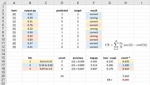 [Click on image for larger view.] Figure 1: Calibration Error for a Binary Classifier
The number of bins to use is arbitrary to some extent. Suppose you decide to use B = 3 equal-interval bins. Therefore, bin 1 is for computed output pseudo-probabilities from 0.0 to 0.33, bin 2 is for 0.34 to 0.66, bin 3 is for 0.67 to 1.0. Each data item is associated with the bin that captures the item's pseudo-probability. So, bin 1 contains items [2] and [4], bin 2 contains items [0], [1], [5], [8] and [9], and bin 3 contains items [3], [6] and [7].
For each bin, you calculate the model accuracy for the items in the bin, and the average pseudo-probability of the items in the bin. For bin 1, item [2] is correctly predicted but item [4] is incorrectly predicted. Therefore the accuracy of bin 1 is 1/2 = 0.500. Similarly, the accuracy of bin 2 is 4/5 = 0.800 and the accuracy of bin 3 is 2/3 = 0.667.
For bin 1, the average of the pseudo-probabilities is (0.31 + 0.22) / 2 = 0.265. The average of the pseudo-probabilities in bin 2 is (0.61 + 0.39 + 0.59 + 0.57 + 0.41) / 5 = 0.514. The average pseudo-probability for bin 3 is (0.76 + 0.92 + 0.83) / 3 = 0.837.
Next, the absolute value of the difference between model accuracy and average pseudo-probability is calculated for each bin. At this point, the calculations are:
bin                 acc    avg pp  |diff|
 1   0.00 to 0.33   0.500  0.265   0.235
 2   0.34 to 0.66   0.800  0.514   0.286
 3   0.67 to 1.00   0.667  0.837   0.170
You could calculate a simple average of the bin differences, but because each bin has a different number of data items, a better approach is to calculate a weighted average. So, the final calibration error value is calculated as:
CE = [(2 * 0.235) +  (5 * 0.286) + (3 * 0.170)] / 10
   = (0.470 + 1.430 + 0.510) / 10
   = 2.410 / 10
   = 0.241
Notice that if each bin accuracy equals the associated average pseudo-probability, the calibration error is zero. Larger differences between bin accuracy and average pseudo-probability give larger calibration error.
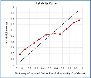 [Click on image for larger view.] Figure 2: A Calibration Reliability Curve
A model's calibration error is sometimes displayed as a reliability curve graph such as the one shown in Figure 2. The graph represents a model where CE has been calculated using 10 bins. It is standard practice to place average bin pseudo-probabilities (confidence) on the x-axis and model bin accuracy on the y-axis. The closer the curve lies to the dashed accuracy-equals-confidence line, the more well-calibrated the model is. Instead of using a line graph, the confidence and accuracy data can be displayed using a histogram; this format is called a reliability diagram.
The calibration error metric is simple and intuitive. But CE has some weaknesses. The number of bins to use is somewhat arbitrary, and with equal-interval bins, the number of data items in each bin could be significantly skewed. There are several variations of the basic CE metric, for example, using bins with equal counts of data items.
Measuring Calibration Error for a Multi-Class Classification Model
There are many ways to measure calibration error for a multi-class classification model. The simplest technique is to extend basic binary classification calibration error to handle multiple classes. This metric is called Expected Calibration Error (ECE).
Suppose you have a problem where the goal is to predict the credit worthiness (0 = poor, 1 = average, 2 = good, 3 = excellent) of a loan applicant based on their income, gender, debt, and so on. And suppose you create a neural network classifier. For a given set of input predictor values, the raw output of the neural network will be a vector with four values, such as (-1.03, 3.58, 0.72, -0.85). The raw output values are called logits. The zero-based index location of the largest logit value indicates the predicted class. Here, the largest value is 3.58 at [1] so the predicted class is 1 = average credit worthiness.
At some point during or after network training, the logit values are scaled to values that sum to 1.0 so that they can be compared to a target vector like (0, 1, 0, 0). The scaling is done directly using a function called softmax or indirectly using log-softmax. For the four logits of (-1.03, 3.58, 0.72, -0.85), the scaled pseudo-probabilities are (0.009, 0.927, 0.053, 0.011). The largest value is still at index [1] and so the predicted class is 1 as it was when determined using the logit values.
Neural network multi-class classifiers are sometimes not well-calibrated. For this example, the model accuracy of class 1 is almost certainly less than the computed pseudo-probability of 0.927, and the model accuracies of class 0, 2 and 3 are likely greater than 0.009, 0.053 and 0.011.
The process for computing expected calibration error for a multi-class model is nearly the same as computing binary classification calibration error. The main difference is that for a multi-class model, each data item generates multiple pseudo-probabilities instead of just a single pseudo-probability. In ECE you simply use the largest pseudo-probability and ignore the others. The spreadsheet shown in Figure 3 shows a worked example of ECE for a multi-class classifier.
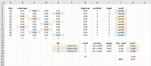 [Click on image for larger view.] Figure 3: Expected Calibration Error for Multi-Class Classification
Compared to alternative measures of calibration error, three advantages of ECE are:
- It's simple to calculate
- It's intuitive
- It's commonly used so it acts as a de facto baseline
Three disadvantages of ECE are:
- The number of bins is arbitrary
- Equal-interval bins can be skewed with regards to data item counts
- By using just the largest output pseudo-probability, some information is being lost
Many alternatives to the ECE metric exist and address one or more of ECE's disadvantages, at the cost of increased metric complexity. Examples include static calibration error (SCE), adaptive calibration error (ACE), and thresholded adaptive calibration error (TACE).
Temperature Scaling for Model Calibration
There are dozens of techniques to deal with ML models that are not well-calibrated. Most of these techniques fall into one of two categories:
- Techniques applied during model training that attempt to prevent miscalibration from occurring
- Model-augmentation techniques applied after model training to create a new, better-calibrated model
A review of research literature indicates that one of the most common and effective techniques used in practice is called temperature scaling. It is a model-augmentation approach.
Temperature scaling is best explained by using a concrete example. The idea of temperature scaling is almost too simple: before scaling raw output logit values with softmax, all output logit values are divided by a numeric constant called the temperature (T).
Suppose you have a classification model that predicts one of three classes. You compute the ECE for the trained model and determine that the model is not well-calibrated. If the logit output values for a data item are (-1.50, 2.00, 1.00), then without temperature scaling the output pseudo-probabilities from softmax are (0.022, 0.715, 0.263).
If the value of the temperature scaling factor is T = 1.5, then you'd divide the three logits by T giving (-1.00, 1.33, 0.67). Now, when you apply softmax, the modified output pseudo-probabilities are (0.060, 0.621, 0.319). Notice that the original pseudo-probability value of 0.715 for predicted class 1 has been reduced to 0.621 and the original pseudo-probabilities of 0.022 and 0.263 for classes 0 and 2 have been increased to 0.060 and 0.319. The value of T isn't arbitrary -- it has been calculated so that the new pseudo-probabilities are closer to model accuracies.
Notice that dividing logits by a constant doesn't change the index location of the largest value. Therefore, using temperature scaling does not change which class is predicted by a neural network, and so temperature scaling calibration doesn't affect model prediction accuracy.
This is all very simple, but where does the value of the temperature scaling constant T come from? When training a neural network, the most common technique is to use some form of calculus stochastic gradient descent (SGD). SGD iteratively modifies the values of the weights and biases that define the network's behavior so that output values closely match target values, as measured by some form of error, typically mean squared error or cross entropy error. Put another way, if you have known target values and an error function, you can use an optimization algorithm to find the best values of the network's weights.
In the much same way, to find the value of the single temperature scaling constant T you can use a set of held-out validation data and run an auxiliary program that starts with an existing model and optimizes the value of T using expected calibration error and SGD or a similar optimizing algorithm.
The main advantage of temperature scaling calibration is that it's relatively simple. The two main disadvantages are that temperature scaling requires a relatively large extra set of validation data beyond training and test data, and the quality of the calibrated model depends entirely on how representative the validation data is.
Wrapping Up
One of the main reasons for the increased interest in machine learning model calibration is the fact that the more complex a model is, the more likely the model is to not be well-calibrated. For example, the five-layer LeNet deep neural image classification model, which was a breakthrough in 1998, is quite well-calibrated on the CIFAR-100 benchmark dataset, with an ECE of approximately 0.05. However, the 110-layer ResNet model, which was state-of-art in 2016, is not well-calibrated with an ECE of approximately 0.20 on the same dataset.