In-Depth
Researchers Explore Bayesian Neural Networks
At first thought, Bayesian neural networks don't seem to make much sense. So what are they and why is there such great interest in them?
- By Pure AI Editors
- 09/07/2021
The agenda of the recently completed 2021 International Conference on Machine Learning (ICML) lists over 30 presentations related to the topic of Bayesian neural networks. What are Bayesian neural networks and why is there such great interest in them?
A standard neural network has a set of numeric constants called weights and special weights called biases. For a given input, a standard neural network uses the values of the weights and biases, and the input, to compute an output value. For a specific input, a standard neural network will produce the same result every time.
The term "Bayesian" loosely means "based on probability." A Bayesian neural network (BNN) has weights and biases that are probability distributions instead of single fixed values. Each time a Bayesian neural network computes output, the values of the weights and biases will change slightly, and so the computed output will be slightly different every time. To make a prediction using a BNN, one approach is to feed the input to the BNN several times and average the results.
At first thought, Bayesian neural networks don't seem to make much sense. However, BNNs have two advantages over standard neural networks. First, the built-in variability in BNNs makes them resistant to model overfitting. Model overfitting occurs when a neural network is trained too well. Even though the trained model predicts with high accuracy on the training data, when presented with new previously unseen data, the overfitted model predicts poorly. A second advantage of Bayesian neural networks over standard neural networks is that you can identify inputs where the model is uncertain of its prediction. For example, if you feed an input to a Bayesian neural network five times and you get five very different prediction results, you can treat the prediction as an "I'm not sure" result.
Bayesian neural networks have two main disadvantages compared to standard neural networks. First, BNNs are significantly more complex than standard neural networks, which makes BNNs difficult to implement. Second, BNNs are more difficult to train than standard neural networks. Much of the current research related to Bayesian neural networks is related to finding techniques to make them easier to train.
Understanding How Bayesian Neural Networks Work
Bayesian neural networks are best explained using an analogy example. Suppose that instead of a neural network, you have a prediction equation y = (8.5 * x1) + (9.5 * x2) + 2.5 where y is the predicted income of an employee, x1 is normalized age, and x2 is years of job tenure. The predicted income of a 30-year old who has been on the job for 4 years would be y = (8.5 * 3.0) + (9.5 * 4.0) + 2.5 = 64.5 = $64,500. If you feed the same (age, tenure) input of (3.0, 4.0) to the prediction equation, you will get the same result of 64.5 every time. The w1 = 8.5 and w2 = 9.5 constants are the prediction equation weights and the b = 2.5 constant is the bias.
Now suppose that instead of fixed weights of (w1 = 8.5, w2 = 9.5) and bias of b = 2.5, the prediction equation uses probability distributions. For example, perhaps the age weight w1 is Gaussian (Normal, bell-shaped) with mean = 8.5 and standard deviation = 1.0, and the tenure weight w2 is Gaussian with mean = 9.5 and standard deviation = 1.5, and the bias b is Gaussian with mean = 2.5 and standard deviation = 0.4. This could be expressed more compactly as w1 = (N, 8.5, 1.0), w2 = (N, 9.5, 1.5), b = (N, 2.5, 0.4).
If you feed input of (age = 3.0, tenure = 4.0) to the Bayesian prediction equation three times, you will get three different results, such as:
1: (w1 = 8.4, w2 = 9.7, b = 2.4) : y = 65.0 = $65,000
2: (w1 = 8.7, w2 = 9.1, b = 2.6) : y = 63.5 = $63,500
3: (w1 = 8.5, w2 = 9.3, b = 2.7) : y = 63.7 = $63,700
Because the weights and bias are sampled from probability distributions, their values will change on each sample. On the first call to the prediction equation, the sampled age weight was 8.4 (slightly less than the distribution mean of 8.5), the tenure weight was 9.7 (slightly greater than the mean of 9.5) and the bias was 2.4 (slightly less than the mean of 2.5). The average predicted income of the employee is $64,070. The graph in Figure 1 shows a Gaussian distribution with mean = 8.5 and standard deviation = 1.0. Most sampled values will be close to 8.5 and almost all will be between 5.5 and 11.5.
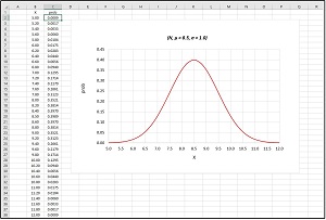 [Click on image for larger view.] Figure 1: TGaussian distribution with mean = 8.5 and standard deviation = 1.0.
Bayesian neural networks are conceptually similar to this prediction equation example. The main difference is that a neural network has many weights and biases and the output is computed using more complex math. A standard neural network must be trained to find the values of the weights and biases. This is usually done by comparing computed output values with known correct output values contained in a set of training data, and computing error/loss. This is fairly difficult.
A Bayesian neural network that uses Gaussian distributions for the weights and biases must be trained to find the means and standard deviations for each distribution. This is more difficult. The training process to find the distribution means and standard deviations typically involves comparing probability distributions using a function called the Kullback-Leibler divergence.
 [Click on image for larger view.] Figure 2: An example of a Bayesian neural network in action.
The screenshot in Figure 2 shows an example of a Bayesian neural network in action on the well-known Iris Dataset. The goal is to predict the species (0 = setosa, 1 = versicolor, 2 = virginica) of an iris flower based on sepal length and width, and petal length and width. A sepal is a leaf-like structure. After the Bayesian neural network was trained, it was fed an input of [5.0, 2.0, 3.0, 2.0] three times. The first output was [0.0073, 0.8768, 0.1159]. These are probabilities of each class. Because the largest probability value is 0.8768 at index [1], the prediction is class 1 = versicolor. The other two outputs were similar.
Recent Research on Bayesian Neural Networks
The 2021 ICML virtual event was held July 18-24. A search for "bayesian neural" returned over 30 presentations. A brief summary of four of these presentations provides a glimpse into current research on Bayesian neural networks. The two images in Figure 3 are representative pages from the presentations. The point is that research targets a very small group of people with deep mathematical backgrounds and so there is a significant barrier for translating the ideas of research into practical engineering systems that solve real-world problems.
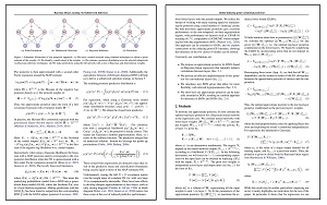 [Click on image for larger view.] Figure 3: Two representative pages from recent research on Bayesian neural networks.
- The paper "Bayesian Deep Learning via Subnetwork Inference" by E. Daxberger, E. Nalisnick, J. Allingham, J. Antoran and J. Hernandez-Lobato addresses the difficulty of training. The abstract, in part, is: "The Bayesian paradigm has the potential to solve core issues of deep neural networks such as poor calibration and data inefficiency. Alas, scaling Bayesian inference to large weight spaces often requires restrictive approximations. In this work, we show that it suffices to perform inference over a small subset of model weights in order to obtain accurate predictive posteriors."
- The paper "What Are Bayesian Neural Network Posteriors Really Like?" by P. Izmailov, S. Vikram, M. Hoffman and A. Wilson addresses ideas to improve the predictive accuracy of Bayesian neural networks. The beginning of the abstract is: "The posterior over Bayesian neural network (BNN) parameters is extremely high-dimensional and non-convex. For computational reasons, researchers approximate this posterior using inexpensive mini-batch methods such as mean-field variational inference or stochastic-gradient Markov chain Monte Carlo (SGMCMC). To investigate foundational questions in Bayesian deep learning, we instead use full batch Hamiltonian Monte Carlo (HMC) on modern architectures."
- The paper "Global Inducing Point Variational Posteriors for Bayesian Neural Networks and Deep Gaussian Processes" by S. Ober and L. Aitchison explores the behavior of Bayesian neural networks. The first two sentences of the abstract are: "We consider the optimal approximate posterior over the top-layer weights in a Bayesian neural network for regression, and show that it exhibits strong dependencies on the lower-layer weights. We adapt this result to develop a correlated approximate posterior over the weights at all layers in a Bayesian neural network."
- The paper "Are Bayesian Neural Networks Intrinsically Good at Out-of-Distribution Detection?" by C Henning, F. D'Angelo and B. Grewe looks at the ability of Bayesian neural networks to identify "I'm not sure" prediction scenarios. "The need to avoid confident predictions on unfamiliar data has sparked interest in out-of-distribution (OOD) detection. It is widely assumed that Bayesian neural networks (BNN) are well suited for this task, as the endowed epistemic uncertainty should lead to disagreement in predictions on outliers. In this paper, we question this assumption and provide empirical evidence that proper Bayesian inference with common neural network architectures does not necessarily lead to good OOD detection."