Researchers Explore Differential Evolution Optimization for Machine Learning -- Pure AI

Researchers Explore Differential Evolution Optimization for Machine Learning

Differential evolution may allow the creation of neural prediction systems that are more powerful than the current generation of systems.

By Pure AI Editors
08/02/2021

Researchers at Microsoft have demonstrated that a technique called differential evolution can be used to train deep neural networks. Differential evolution is a specific form of an evolutionary algorithm -- an algorithm based on biological processes such as mating and natural selection. Differential evolution may allow the creation of neural prediction systems that are more powerful than the current generation of systems.

Training a neural network is the process of finding values for the network's weights and biases (biases are a special type of weight). Deep neural networks can have billions of weights and training can take weeks or months, and cost millions of dollars in compute resources. Most production systems train neural networks using a technique called stochastic gradient descent (SGD). SGD optimization has many variations and modifications with names such as Adam (adaptive momentum estimation) and Adagrad (adaptive gradient).

All forms of SGD training use the Calculus derivative of an error function. Training neural networks with forms of SGD is often highly effective but the approach has two weaknesses. First, neural network architectures can only use relatively simple internal functions that are mathematically differentiable. Second, training very deep neural networks with SGD often runs into a problem called the vanishing gradient, when training stalls and no progress can be made.

Understanding Differential Evolution Optimization
Training a neural network is a type of mathematical minimization optimization problem. The goal is to find the values for network weights that minimize the error between network computed output values and known correct output values contained in a set of training data. There are many types of optimization algorithms that don't rely on the use of Calculus gradients. One category of non-gradient techniques is called evolutionary algorithms. An evolutionary algorithm is any algorithm that loosely mimics biological evolutionary mechanisms such as mating, chromosome crossover, mutation, and natural selection.

A generic form of a standard evolutionary algorithm is:


    create a population of possible solutions
    loop
      pick two good solutions
      combine them using crossover to create child
      mutate child slightly
      if child is good then
        replace a bad solution with child
      end-if
    end-loop
    return best solution found

Standard evolutionary algorithms can be implemented using dozens of specific techniques. Differential evolution is a special type of evolutionary algorithm that has a relatively well-defined structure:

create a population of possible solutions
loop
  for-each possible solution
    pick three other random solutions
    combine the three to create a mutation
    combine curr solution with mutation = candidate
    if candidate is better than curr solution then
      replace current solution with candidate
    end-if
  end-for
end-loop
return best solution found

The "differential" term in "differential evolution" is a rather unfortunate choice. Differential evolution does not use derivatives, gradients, or anything related to differential Calculus. The "differential" refers to a specific part of the algorithm where three possible solutions are combined to create a mutation, based on the difference between two of the possible solutions.

An Example of Differential Evolution Optimization
Differential evolution is best explained by example. Suppose the function to minimize is the simple sphere function in five dimensions: f(x0, x1, x2, x3, x4) = x0^2 + x1^2 + x2^2 + x3^2 + x4^2. The function has an obvious minimum at (0, 0, 0, 0, 0) when the value of the function is 0.0. The sphere function in 2D is shown in Figure 1. The function gets its name from the fact that its shape is spherical in 2D.

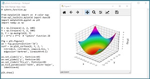Figure 1: The sphere function for dimension = 2. — **[Click on image for larger view.]** **Figure 1:** The sphere function for dimension = 2.

An example of differential evolution to solve the sphere function in 5D is illustrated in Figure 2. The algorithm begins by creating a population of eight possible solutions. Each initial possible solution is randomly generated. Larger population sizes increase the chance of getting a good result at the expense of computation time. Each possible solution has an associated error. The first possible solution, x[0] = (-1.3, 4.6, 2.7, -3.2, 3.5), has an absolute error of 52.63 because -1.3^2 + 4.6^2 + 2.7^2 + -0.2^2 + 3.5^2 = 52.63.

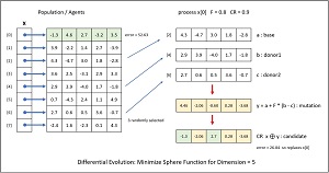Figure 2: One iteration of differential evolution optimization. — **[Click on image for larger view.]** **Figure 2:** One iteration of differential evolution optimization.

Each of the eight possible solutions is processed one at a time. First, three of the other possible solutions are randomly selected and labeled a, b, c. In the example, items [2], [4], and [6] were selected. Next, items a, b and c are combined into a mutation using the equation y = a + F * (b - c). The F is the "differential weight" and is a value between 0 and 2 that must be specified. In the example, F = 0.80.

The calculations for the mutation y are:

(b-c) =  (2.9, 3.9, -4.0, 1.7, -1.8)
       - (2.7, 0.6,  0.5, 3.6, -0.7)
      
      =  (0.2, 3.3, -4.5, -1.9, -1.1)

F * (b-c) = 0.8 * (0.2, 3.3, -4.5, -1.9, -1.1)
          = (0.16, 2.64, -3.60, -1.52, -0.88)

a + F * (b - c) =  (4.3,  -4.7,   3.0,   1.8,  -2.8)
                 + (0.16,  2.64, -3.60, -1.52, -0.88)

                =  (4.46, -2.06, -0.60,  0.28, -3.68)

Next, the mutation y is combined with the current possible solution x[0] using crossover to give a candidate solution. Each cell of the candidate solution takes the corresponding cell value of the mutation with probability CR (crossover rate) -- usually, or the value of the current possible solution with probability 1-CR (rarely). In the example, CR is set to 0.9 and by chance, the candidate solution took values from the mutation at cells [1], [3], [4], and took values from the current possible solution at cells [0], [2]:

current:   (-1.3,   4.6,   2.7,  -3.2,   3.5)
mutation:  ( 4.46, -2.06, -0.60,  0.28, -3.68)
candidate: (-1.3,  -2.06,  2.7,   0.28, -3.68)

The last step is to evaluate the newly generated candidate solution. In this example the candidate solution has absolute error = -1.3^2 + -2.06^2 + 2.7^2 + 0.28^2 + -3.68^2 = 26.84. Because the error associated with the candidate solution is less than the error of the current possible solution (52.63), the current possible solution is replaced by the candidate. If the candidate solution had greater error, no replacement would take place.

To summarize, each possible solution in a population is compared with a new candidate solution. The candidate is generated by combining three randomly selected possible solutions (a mutation) and then combining the mutation with the current possible solution (crossover). If the candidate replaces the current solution if the candidate is better.

Note that the terminology of differential evolution optimization varies quite a bit from research paper to paper. For example, the possible solutions are sometimes called agents, and the term mutation is used in different ways. And there are many variations of basic differential evolution. For example, in some versions of differential evolution, one cell from the mutation is guaranteed to be used in the candidate.

Applying Differential Evolution to Neural Network Training
Differential evolution optimization is most often used for electrical engineering problems. Researchers at Microsoft applied differential evolution to neural network training. When used for standard neural network problems, such as MNIST handwritten digit recognition, differential evolution training performed comparably to stochastic gradient descent training. Dr. James McCaffrey commented, "For most neural scenarios, differential optimization doesn't provide enough advantage to warrant using it instead of classical gradient-based training algorithms."

He added, "However, my colleagues and I think that differential evolution may eventually be valuable in two scenarios. First, very deep neural systems, such as Transformer Architecture systems used for natural language processing, may eventually reach a size where they're no longer trainable using gradient-based techniques. Second, differential evolution may allow the creation of new types of powerful neural systems -- those that use sophisticated non-differentiable functions in hidden layers."

McCaffrey observed, "The biggest disadvantage of differential evolution is performance. Differential evolution training typically takes much longer than gradient-based training. However, at some point in the future, quantum computing may open the door for differential evolution and similar algorithms to revolutionize predictive systems."