How-To
Comparing 4 ML Classification Techniques: Logistic Regression, Perceptron, Support Vector Machine, and Neural Networks
Learn about four of the most commonly used machine learning classification techniques, used to predict the value of a variable that can take on discrete values.
- By Pure AI Editors
- 04/15/2020
In machine learning and artificial intelligence, an important type of problem is called classification. This article describes and compares four of the most commonly used classification techniques: logistic regression, perceptron, support vector machine (SVM), and single hidden layer neural networks.
The goal of a classification problem is to predict the value of a variable that can take on discrete values. In binary classification the goal is to predict a variable that can be one of just two possible values, for example predicting the gender of a person (male or female). In multi-class classification the goal is to predict a variable that can be three or more possible values, for example, predicting a person's state of residence (Alabama, Alaska, . . . Wyoming). Note that a regression problem is one where the goal is to predict a numeric value, for example the annual income of a person.
There are dozens of ML classification techniques, and most of these techniques have several variations. One way to mentally organize ML classification techniques is to place each into one of three categories: math equation classification techniques, distance and probability classification techniques, and tree classification techniques.
This article explains four of the most common math equation classification techniques: A future PureAI article will explain compare common distance and probability techniques (k-nearest neighbors and naive Bayes), and common tree techniques (decision tree, bootstrap aggregation, random forest, and boosted trees).
Classification is called a supervised technique. This means that a prediction model is created using data that has known, correct input and output values. This data is called training data, or sometimes reference data. The term supervised is used to distinguish classification from machine learning techniques that don't require training data, in particular clustering techniques such as k-means and Gaussian mixture model.
Because classification is used by many different disciplines, there are several terms used for each idea. For example, predictor variables are also known as features (data science), signals (electrical engineering), attributes (social sciences), and independent variables (mathematics). The variable to predict is also known the class, or the label, or the dependent variable.
Logistic Regression Example
Suppose you want to predict the gender (male = 0, female = 1) of a person based on their age, height, and income. To make the prediction, you compute a weighted sum of products of the predictor values, and then apply the logistic sigmoid function to the sum to get a p-value. The p-value will be between 0.0 and 1.0 and if it's less than 0.5 the prediction is class 0 (male) and if the p-value is greater than or equal to 0.5 the prediction is class 1 (female).
Imagine you have a person with age = x0 = 0.30 (i.e., 30 years old), height = x1 = 0.66 (66 inches), and income = x2 = 0.54 ($54,000.00). A logistic regression model will have three weights, w0, w1, w2, and a special weight called a bias, b. Suppose the values of the weights and the bias are w0 = 1.5, w1 = 1.1, w2 = 1.8, b = -2.8. The intermediate weighted sum of products value (often called z) is:
z = (w0 * x0) + (w1 * x1) + (w2 * x2) + b
  = (0.30 * 1.5) + (0.66 * 1.1) + (0.54 * 1.8) + (-2.8)
  = -0.65
The logistic sigmoid function of any value x is 1 / (1 + exp(-x)) where the exp() function is a core math function that you can think of as a black box. Therefore, the computed p-value for the example is:
p = 1 / (1 + exp(+0.65))
  = 1 / (1 + 1.92)
  = 0.34
Because the p-value is less than 0.5, the prediction is class 0 (male). Note that the term logistic regression is a bit confusing because LR is a classification technique but LR works by generating a single numeric value.
The difficult part of creating a logistic regression model is determining the values of the weights and the bias. This is called training the model. To train, you use a set of data that has known predictor values and known, correct class labels (the value to predict). You must use an optimization algorithm to examine different values of the weights and the bias, looking for values so that the precited class labels most closely match the correct target values.
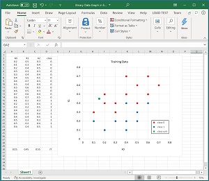 [Click on image for larger view.] Figure 1: Some Dummy Training Data
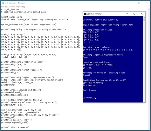 [Click on image for larger view.] Figure 2: Logistic Regression Using the scikit Code Library
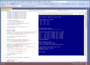 [Click on image for larger view.] Figure 3: Logistic Regression Using Raw C# Code
There is no closed form solution for finding the best values for the weights and the bias. A major source of confusion for people who are new to ML is that there are at least a dozen different algorithms that can be used for logistic regression training, and each algorithm has many variations. Put another way, there are many math equation classification techniques. Each of these classification techniques requires training to find the values of the weights and the bias, and there are many of these training optimization algorithms.
Five of the most commonly used types of optimization algorithms for training are gradient descent (techniques that iteratively reduce error), gradient ascent (techniques that iteratively increase likelihood), iterated Newton-Raphson (a technique that uses matrix operations), L-BFGS (a technique that uses classical statistics ideas), and evolutionary optimization (techniques that loosely model biological processes).
The images in
Figures 1, 2 and 3 illustrate what logistic regression looks like in action.
Figure 1 shows a graph of some hypothetical training data. There are three predictor variables but only the first two are shown on the graph.
Figure 2 shows an example of logistic regression on the data using the scikit Python code library.
Figure 3 shows an example on the same data using custom C# code from scratch (no external libraries).
Perceptron Example
Suppose you want to predict whether a banknote (think dollar bill or euro) is authentic (class -1) or a forgery (class +1) based on characteristics of a digital image of the banknote: variance, kurtosis, and entropy. To make the prediction, you compute a weighted sum of products of the predictor values, and then apply the skewed signum function to the sum to get an s-value. The s-value will be either -1 or +1 and gives you the predicted class.
Imagine you have a banknote with variance = x0 = -0.95, kurtosis = x1 = 0.44, and entropy = x2 = -0.67. A perceptron model will have three weights, w0, w1, w2, and a special weight called a bias, b. Suppose the values of the weights and the bias are w0 = 3.9, w1 = 2.3, w2 = 1.2, b = 2.1. The intermediate weighted sum of products value (sometimes called z) is:
z = (w0 * x0) + (w1 * x1) + (w2 * x2) + b
  = (-0.95 * 3.9) + (0.44 * 2.3) + (-0.67 * 1.2) + 2.1
  = -1.39
The skewed signum function of any value x is -1 if x is negative or +1 if x is positive or zero. Therefore, the s-value ("sign value") is:
s = signum(-1.39)
  = -1
Because the s-value for the example is -1 the prediction is class -1 (authentic).
Perceptron classification is simple and relatively crude. Common optimization algorithms for training a perceptron classifier include gradient descent, gradient ascent, simplex, and L-BFGS. A minor variation used for training a perceptron classifier averages model weights and the bias; when used the resulting prediction model is sometimes called an averaged perceptron.
Support Vector Machine Example
Suppose you want to predict if a patient has heart disease or not (class -1 = absence of disease, class +1 = presence of disease) based on blood pressure, cholesterol level, and heart rate. To make a prediction you examine your training data to find two key data items that separate the class 0 items from the class 1 items in a subtle optimal way. These two key items are called the support vectors. A vector is a point with three or more values, such as (1.5, 7.3, 2.9).
The two support vectors determine a decision boundary line (technically a hyperplane when there are three or more predictor variables). The decision line/hyperplane is a math equation with three coefficients (one per predictor variable) and a constant called the intercept. The output of the decision equation will be a numeric value from negative infinity to positive infinity. If the output value is negative, the prediction is class -1 and if the output value is positive or zero, the prediction is class +1.
Imagine you have a patient with blood pressure = x0 = 0.78, cholesterol = x1 = -0.63, and heart rate = x2 = 0.54. Suppose the two support vectors determine a hyperplane decision equation defined by coefficients w0 = 4.5, w1 = 5.2, w2 = 3.8, and b = 2.7 and so the decision equation is y = (4.5 * x0) + (5.2 * x1) + (3.8 * x2) + 2.7.
For the given patient, the value of the decision equation is:
y = (4.5 * 0.78) + (5.2 * -0.63) + (3.8 * 0.54) + 2.7
  = 4.98
Because the value of the decision equation is positive, the predicted class is +1 (presence of heart disease).
This example is deceptive because it makes SVM appear simpler than it really is. Once the decision hyperplane equation is determined, making a prediction is very simple. But training an SVM classifier involves first finding the two key support vectors and then using them to determine the equation of the decision hyperplane. Both parts of the training process are very complicated and require dedicated, highly specialized, complex optimization algorithms.
The word "machine" in the term "support vector machine" is an unfortunate translation from the original Russian research paper that first described the classification technique. A better translation might have been "support vector classifier."
Neural Network Example
Suppose you want to predict if an object on the ocean floor is a rock (class 0) on a mine (class 1) based on sonar readings of the object taken from angles of 30 degrees, 60 degrees, and 90 degrees. To make the prediction, you could construct a 3-4-1 neural network (three input nodes, four hidden processing nodes, one output node). The neural network will compute a single value between 0.0 and 1.0 and store it in the output node. If the output node value is less than 0.5 the prediction is class 0 (rock) and if the output node value is greater than or equal to 0.5 the prediction is class 1 (mine).
The number of input nodes and output nodes is determined by the problem data but the number of hidden nodes is a hyperparameter, meaning it's a value that must be determined by trial and error. Another term for hyperparameter is free parameter, meaning it can be freely chosen.
Unlike logistic regression, perceptron, and support vector machine classifiers, which are designed only for binary classification, neural network classifiers can easily be extended to handle multi-class classification problems by adding output nodes. For example, if you had a problem where you wanted to predict the political leaning of a person and the possible values are (conservative, moderate, liberal), then you would create a neural network with three output nodes. In other words, for binary classification a neural network has one output node. For multi-class classification a neural network has n output nodes where n is the number of possible values to predict.
A neural network has a weight associated with each input-hidden connection and each hidden-output connection, and has a bias for each hidden and each output node. If a neural network has ni input nodes, nh hidden nodes, and no output nodes, it will have (ni * nh) + (nh * no) weights and nh + no biases. For example, a 3-4-1 neural network binary classifier will have (3 * 4) + (4 * 1) + (4 + 1) = 21 weights and biases. If you have four predictor variables and three possible values to predict, a 4-7-3 neural network multi-class classifier would have (4 * 7) + (7 * 3) + (7 + 3) = 59 weights and biases.
For the 3-4-1 rock-mine example, to make a prediction the first step is to use the predictor values and the input-hidden weights and the hidden node biases to compute the values of the four hidden nodes:
h0 = tanh(  (ih00 * x0) + (ih10 * x1) + (ih20 * x2) + hb0 )
h1 = tanh(  (ih01 * x0) + (ih11 * x1) + (ih21 * x2) + hb1 )
h2 = tanh(  (ih02 * x0) + (ih12 * x1) + (ih22 * x2) + hb2 )
h3 = tanh(  (ih03 * x0) + (ih13 * x1) + (ih23 * x2) + hb3 )
In words, the value of a hidden node is the hyperbolic tangent applied to the sum of products of weights and predictor values plus the bias. The tanh function is similar to the logistic sigmoid function, except that tanh returns a value between -1.0 and +1,0 instead of 0.0 and 1.0.
At this point each hidden node will have a value. The second step to make a prediction is to compute the value of the output node:
out0 = logsig( (ho00 * h0) + (ho10 * h1) + (ho20 * h2) + (ho30 * h3) + ob0 )
If there are three or more output nodes for a multi-class neural classifier, when computing the values of the output nodes, you use a function called the softmax function instead of the logistic sigmoid function. The result will be a set of values that sum to 1.0 and can be interpreted as the probability of each class. For example, if there are three possible class values, 0, 1, 2, and the neural network output node values are (0.25, 0.65, 0.10), the prediction is class 1 because it has the largest probability.
Training a neural network to find the values of the weights and biases is a difficult challenge. Although there are many possible optimization algorithms that can be used, the most common is a version of gradient descent called stochastic gradient descent. When stochastic gradient descent (usually abbreviated as SGD) is used to train a neural network, the algorithm is often called back-propagation.
Common Themes for Machine Learning Classification
There are six issues that are common to math equation classification techniques such as logistic regression, perceptron, support vector machine, and neural networks. These six issues are 1.) dealing with model overfitting, 2.) dealing with error, loss, and accuracy, 3.) dealing linearly separable data, 4.) dealing with varying magnitude numeric predictor variables, 5.) dealing with non-numeric predictor variables, and 6.) dealing with multi-class classification problems. Most of these six issues are also applicable to other classification techniques such as distance and probability techniques, and techniques based on decision trees, but the impact of these six issues is either somewhat different or isn't as important.
In addition to the six issues for math equation classification, there are three issues that are common to all machine learning classification techniques: 7.) dealing with training and test data, 8.) dealing with interpretability, and 9.) dealing with implementation and integration.
1. Dealing with Overfitting
When using math equation classification techniques, a major challenge is called overfitting. Overfitting occurs when you train a model for too long; the resulting model predicts very well for the training data but when presented with new, previously unseen data the model predicts poorly.
There are many ways to deal with overfitting. One of the most common is called regularization. A symptom of overfitted math equation models is weight values that are very large in magnitude. Regularization limits the magnitudes of model weights. There are several forms of regularization; the two most common are called L1 and L2 regularization. A technique called elastic-net regularization is essentially a combination of L1 and L2 regularization.
A machine learning classification model that hasn't been trained enough and gives poor prediction accuracy is said to be underfitted.
2. Dealing with Error, Accuracy, and Loss
When training a math equation classification model, most optimization algorithms try to reduce the error measured by comparing computed output values with correct target values. For example, in logistic regression classification if you have just three training items and at some point during training, suppose the model's current weights and bias give these results:
computed  correct
 0.80      1
 0.30      0
 0.60      1
Notice that the first item is correctly predicted because the computed output is greater than 0.5 which predicts class 1. The second item is also predicted correctly because the computed output is less than 0.5 which predicts class 0. However, the third item is incorrectly predicted. Therefore the current classification accuracy of the model is 2 / 3 = 67 percent accuracy.
Training uses error rather than accuracy. The most common form of error for logistic regression, perceptron, and support vector models is mean squared error. For the data above, the total squared error is (0.80 - 1)^2 + (0.30 - 0)^2 + (0.60 -1)^2 = 0.04 + 0.09 + 0.16 = 0.29 and so the mean squared error is 0.29 / 3 = 0.97.
An alternative form of error that is often used with neural networks is called cross entropy error. For the data above, total cross entropy error is -1 * (1 * log(0.80)) + (0 * log(0.30)) + (1 * log(0.60)) = -1 * ((-0.22) + (-1.20) + (-0.51)) = 1.94 and so the mean cross entropy error is 1.94 / 3 = 0.65.
The error function used during training is sometimes called "loss function" and the corresponding value is called the model loss. Some training algorithms are based on the log of the error value and the term log-loss is used.
3. Dealing with Non-Linearly Separable Data
A serious weakness of the logistic regression, perceptron, and support vector machine classification techniques is that none of them can deal with complex data that is not linearly separable. Neural networks do not have this weakness.
Suppose you have a binary classification problem with two predictor variables. With linearly separable data it's possible to place a straight line (a hyperplane when there are three or more predictor variables) on a graph of the data so that most of the data points representing the first class is on one side of the line/hyperplane and most of the data points representing the second class are on the other side of the line.
In realistic classification scenarios there's no easy way to tell if your data is linearly separable or not. Typically you create a logistic regression or perceptron model and if the model's accuracy on the training data is poor, meaning not much better than just predicting the most common class for every data item, then there's a good chance your data is not linearly separable.
It is possible to extend basic logistic regression, perceptron, and support vector machine classifiers to handle data that is not linearly separable by using what is called the kernel trick. The kernel trick is somewhat complicated. The technique uses what is called a kernel function. Instead of working directly with the original data, kernel techniques apply a kernel function to pairs of data items. The transformed data is mapped to a higher dimension and could be (but isn't guaranteed to be) linearly separable.
Many kernel functions can be thought of as measures of similarity. There are theoretically an infinite number of possible kernel functions, and there are about a dozen commonly used kernel functions. When using the kernel trick, the choice of which kernel function to use, and the values of any of the selected function's parameters, are free parameters that must be determined using trial and error.
A common general purpose kernel function is called the radial basis function (RBF). The function is defined as f(x1, x2) = exp( -1 * || x1 - x2 ||^2 / (2 * s^2) ) where x1 and x2 are two data item vectors, the || operator is the vector norm, and s is a free parameter sometimes called the width. If two vectors x1, and x2 are the same, f(x1, x2) returns 1.0 (maximum similarity) and the more different x1 and x2 are, the closer the return value is to 0.0 (minimum similarity).
In general, machine learning tools and code libraries do not use the kernel trick for logistic regression and perceptron classifiers, but they do use the kernel trick for support vector machine classifiers. But the only way to know for sure if the kernel trick is being used is to read the tool or library documentation.
4. Dealing with Varying Magnitude Numeric Predictor Variables
In practice, when using math equation classifiers, you should normalize the values of the numeric predictor so that the values are all roughly within the same range. This prevents predictor variables with large magnitudes, such as an annual income of $54,000.00, from overwhelming variables with small magnitudes, such as an age of 32.
The three most common types of normalization for predictor variables are divide-by-constant normalization, min-max normalization, and z-score normalization. Suppose you want to predict the gender of a person based on their annual income, age, and job type (mgmt, sales, or tech) and you have three training data items:
income     age job_type  gender
===========================
62,000.00  34  tech      0
46,000.00  40  mgmt      1
72,000.00  28  sales     0
The numeric predictors are income and age. To use divide-by-constant normalize you divide each predictor raw value by the same constant. You could divide all incomes by 100,000 and all ages by 100 giving:
income   age
=============
0.62     0.34
0.46     0.40
0.72     0.28
To use min-max normalization, for each predictor variable you compute x' = (x - min) / (max - min). For example, the income min and max values are 46,000.00 and 72,000.00 so the normalized value of 62,000.00 is (62,000.00 - min) / (max - min) = (62,000.00 - 46,000.00) / (72,000.00 - 46,000.00) = 0.615. The min-max normalized predictor values are:
income   age
==============
0.615    0.500
0.000    1.000
1.000    0.000
To use z-score normalization, for each predictor variable you compute x' = (x - u) / sd where u is the mean of the variable and sd is the standard deviation. For example, the mean of the income values is 60,000.00 and the standard deviation is 10708.25 so the normalized value of 62,000.00 is (62,000.00 - 60,000.00) / 10708.25 = 0.187. The z-score normalized values are:
income   age
===============
 0.187    0.000
-1.307   -1.225
 1.121    1.225
In practice, the type of normalization used usually doesn't have a big impact on the quality of the final trained model. In most situations, data normalization is performed in a preprocessing step before training the model, but some machine learning tools and code libraries can perform normalization on the fly.
5. Dealing with Non-Numeric Predictor Variables
When using math equation classification techniques, after normalizing numeric predictor values, you must convert categorical (non-numeric) predictor values to a numeric form. This is called encoding. The most common form of encoding is called one-hot encoding. The technique is also known as 1-of-N or 1-of-C encoding. Suppose you want to predict the gender of a person based on age, job type (mgmt, sales, tech), and race (white, asian, hispanic, black, other). To encode job type you would set mgmt = (1, 0, 0), sales = (0, 1, 0), and tech = (0, 0, 1). To encode race you would set white = (1, 0, 0, 0, 0), asian = (0, 1, 0, 0, 0), hispanic = (0, 0, 1, 0, 0), black = (0, 0, 0, 1, 0), other = (0, 0, 0, 0, 1).
For binary categorical predictor variables, you can encode using either one-hot encoding or minus-one-plus-one encoding. For example, suppose you have a predictor variable color that can only be one of two possible values, red or blue. You could use one-hot encoding and set red = (1, 0) and blue = (0, 1) or you could use minus-one-plus-one encoding and set red = -1 and blue = +1.
6. Dealing with Multi-Class Classification Problems
Most math equation classification techniques, including logistic regression, perceptron, and support vector machine, are designed primarily for binary classification. It is possible to extend such techniques so that they can handle multi-class classification in two different ways. You can use a technique called one-versus-rest, or you can modify the underlying classification algorithm.
One-versus-rest (OVR), also known as one-versus-all (OVA), is best explained by example. Suppose you have a problem where the goal is to predict a person's job type (actuary, barista, clerk). Using a binary classification technique, such as logistic regression, you'd create three classification models: one for actuary or not-actuary (i.e., barista or clerk), one for barista or not-barista, and one for clerk or not-clerk. Then you'd aggregate the results of the three models to a final prediction. The OVR technique has significant technical and practical problems and is best avoided when possible.
Instead of using OVR, you can make significant changes to a classification technique. Such changes are specific to the type of classification technique and are usually quite complex. The article "How to Do Multi-Class Logistic Regression Using C#" is an example of such a technique-modification approach to convert a binary classification algorithm to a multi-class classification algorithm.
7. Dealing with Training and Test Data
When training a classification model, it's common to split your entire dataset that has known correct values-to-predict into a training dataset (typically about 80 percent of the items) and a test dataset (the remaining 20 percent of the items). Then you train your model using the training data, pretending the test dataset doesn't exist. After training, you compute the trained model's accuracy on the test dataset. If the accuracy of the model on the test dataset is significantly lower than the accuracy of the model on the training dataset, there's a good chance your model is overfitted. The accuracy of the model on the test data is a rough estimation of the accuracy you'd expect on new, previously unseen data.
A related technique is called train-validate-test. You divide your entire dataset into three sets: a training set (typically about 60 percent of the items), validation set (20 percent), and test set (20 percent). You use the training set for training to compute the model weights and bias(es). During training, every so often (typically 10 percent of the iterations) you compute the current model's error and when the error on the validation data starts to increase, you stop training. Then you compute classification accuracy on the test data to see if overfitting occurred or not. The train-validate-test technique is only applicable to those classification techniques where error can be computed, typically math equation techniques. The train-validate-test technique isn't used much anymore because the effort required and the reduction in the number of data items available for training typically isn't worth the improvement in the final trained model.
8. Dealing with Interpretability
There is no widely-accepted formal definition of interpretability. An informal definition is that interpretability is the extent to which a prediction made by a machine learning classification model can be explained to a human. In general, math equation classification techniques are less interpretable than distance and probability classification techniques and decision tree classification techniques. Neural network classifiers are the least interpretable models.
Because math equation techniques involve a sum of products of weights times predictor values, one way to examine interpretability is to compare the magnitudes and the signs of the model weights. For example, in a logistic regression classification model, if the weight associated with one predictor variable is twice as large in magnitude as the weight associated with another predictor, you might be tempted to conclude that the first predictor is more important in some way than the second predictor. Or, if the signs of the weights of two predictors are opposite, then you might suspect that an increase in the value of the first predictor could be compensated by a decrease of the second predictor. However, such interpretations should be used very cautiously because model weight values depend on many complex interacting factors.
A topic that is closely related to interpretability is called counterfactual reasoning. Suppose you have a model that predicts if a loan applicant is a good risk or a bad risk. An example of a counterfactual is, "if your income was $20,000 more and your debt was $5,000 less and your age was 7 years older, then your loan application would have been classified as a good risk instead of a bad risk."
9. Dealing with Implementation and Integration
In general, there are three ways to create a machine learning classification model. You can use an integrated GUI tool such as Weka, you can use a code library such as scikit or ML.NET, or you can write custom code from scratch. Using a comprehensive tool is usually the quickest and easiest approach to create a classification model, but the resulting model is often difficult to integrate into a larger system. Writing code from scratch is usually the most difficult approach to create a classification model, but you have full control over customization and error checking, which allows an efficient and flexible implementation.
An effort to standardize machine learning models so that a model trained using one system can in principle be used by any other system is ONNX (open neural network exchange). As the name suggests, ONNX is intended primarily for neural network models. There is no similar industry-backed standardization effort for non-neural machine learning models.
Wrapping Up
Machine learning classification is a complex topic. Math equation classification techniques assign a weight to each predictor variable, and a standalone weight called a bias. A weighted sum of products of predictor values and weights is computed and then a function such as logistic sigmoid is applied to the sum to determine the predicted class.
Although each individual idea in machine learning classification is relatively simple and easy to understand, there are many ideas involved and the ideas interact in complicated ways. Learning some subjects can be done sequentially. For example, to understand math Calculus, you first learn algebra, then trigonometry, then limits, and so on. But there is no sequential path for mastering machine learning. You must learn in a spiral manner, revisiting topics several times until you reach a solid understanding.