How-To
Computing the Similarity of Machine Learning Datasets
The Pure AI Editors explain two different approaches to solving the surprisingly difficult problem of computing the similarity -- or "distance" -- between two machine learning datasets, useful for prediction model training and more.
- By Pure AI Editors
- 12/01/2020
Researchers at Microsoft have developed interesting techniques for computing the similarity between two machine learning (ML) datasets. Computing the similarity (or dissimilarity or distance) between two datasets is surprisingly difficult.
Knowing the distance between two datasets can be useful for at least two reasons. First, dataset distance can be used for ML transfer learning activities, such as using a prediction model trained on one dataset to quickly train a second dataset. Second, the distance between ML datasets can be useful for augmenting training data -- creating additional synthetic training data which can be used to build a more accurate prediction model.
The details of one of the techniques for computing the distance between two ML datasets are presented in the 2020 research paper "Geometric Dataset Distances via Optimal Transport" by D. Alvarez-Melis and N. Fusi. This first distance metric is called optimal transport dataset distance (OTDD). A different technique for computing dataset difference was developed by J. McCaffrey and S. Chen and has been used internally at Microsoft. This second distance metric is called autoencoded average distance (AAD).
Understanding the Problem
Suppose you have a dataset of images of handwritten digits such as the MNIST (Modified National Institute of Standards and Technology) data. Each image represents a single digit (zero through nine) as 28 x 28 = 784 pixels, where each pixel is a grayscale value between 0 and 255. And suppose you have a second dataset of clothing items such as the Fashion-MNIST data, where each 28 x 28 grayscale image represents one of 10 items: t-shirt, trouser, pullover, dress, coat, sandal, shirt, sneaker, bag, boot. See Figure 1 for examples of MNIST and Fashion-MNIST images. How can you compute a measure of distance between the two datasets?
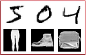 [Click on image for larger view.] Figure 1: Three MNIST images and three Fashion-MNIST images.
The raw data for an MNIST image might look like:
  0  208   67 . . .  145  "five"
167   16  255 . . .   23  "three"
. . .
Each line represents one image. The first 784 values on each line are the pixel values and the last value is the class label. The raw data for Fashion-MNIST could be similar:
110   37  202 . . .   34  "bag"
  7  216   44 . . .  226  "trouser"
. . .
In order to compute the distance between the two datasets, it's necessary to be able to compute the item-item distance between one MNIST item and one Fashion-MNIST item. Computing the distance between the numeric pixel predictor values (often called "features" in ML terminology) is not difficult. The most common technique is to use Euclidean distance. For example, if there were only three pixel values per image, and an MNIST item's pixel values were (25, 0, 100) and a Fashion-MNIST item's pixel vales were (30, 8, 96) then the Euclidean distance between the features, ignoring the class labels, is:
d = sqrt[(25 - 30)^2 + (0 - 8)^2 + (100 - 96)^2)]
  = sqrt(25 + 64 + 16)
  = sqrt(105)
  = 10.25
Computing the Distance Between Class Labels
Unlike numeric data, computing the distance between the non-numeric class labels is not so easy. One approach is to use the Earth Mover's Distance (EMD), also known as the 1-Wasserstein distance. The key idea is to compute the distance between the distributions of the class labels in a way that's analogous to shoveling dirt from several piles into several holes. The technique is best explained by example. See Figure 2.
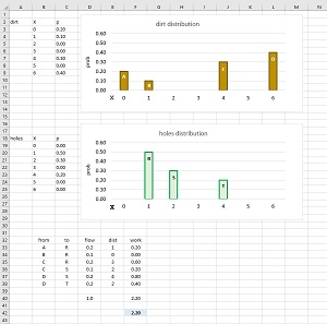 [Click on image for larger view.] Figure 2: Calculating the Earth Mover's Distance / 1-Wasserstein Distance.
Suppose you have two different bizarre dice, each with seven sides labeled "0" through "6". For reasons that will be explained shortly, call the first dice "dirt" and the second dice "holes". You roll the first dirt dice many times and get 20% "0", 10% "1", 30% "4", 40% "6", and 0% for the other three sides. Next, you roll the second holes dice many times and get 50% "1", 30% "2", 20% "4", and 0% for the other four sides. The two frequency distributions are probability distributions because the area of the bars in their graphs sums to 1.
The EMD / 1-Wasserstein distance calculation is a specific type of problem known more generally as OT for "optimal transport". The EMD / 1-Wasserstein distance is the minimal amount of work needed to move the dirt distribution to the holes distribution. Work is defined as the amount of the dirt moved (called flow) times the distance moved. To explain the EMD calculation, the bars in the dirt distribution have been labeled A, B, C, D, and the bars in the holes distribution have been labeled R, S, T.
For this example, the EMD / 1-Wasserstein distance is 2.20 computed in six steps as shown in the bottom part of Figure 2. In words:
1. all 0.2 in A is moved to R, using up A, with R needing 0.3 more.
2. all 0.1 in B is moved to R, using up B, with R needing 0.2 more.
3. just 0.2 in C is moved to R, filling R, leaving 0.1 left in C.
4. all remaining 0.1 in C is moved to S, using up C, with S needing 0.2 more.
5. 0.2 in D is moved to S, filling S, leaving 0.2 left in D.
6. all remaining 0.2 in D is moved to T, using up D, filling T.
With a way to measure the distance between the numeric features of an item and the non-numeric class labels of an item, the distance between two complete items can be computed by a hybrid Euclidean-Wasserstein metric of some sort. The hybrid metric used in the "Geometric Dataset Distances via Optimal Transport" paper is called OTDD for "optimal transport dataset distance".
The OTDD metric uses a variation called 2-Wasserstein rather than basic 1-Wasserstein. In 2-Wasserstein, instead of summing the work = flow * distance values, the distance calculation uses the square root of the sum of the squared work values. And instead of using plain Euclidean distance, the OTDD distance metric uses squared Euclidean distance. The resulting hybrid metric of the distance between two data items has the form distance = sqrt(squared Euclidean distance + 2-Wasserstein distance).
Computing the Distance Between Datasets
After a distance metric between two individual items in different datasets has been defined, the next challenge is to compute an overall distance metric between two datasets. A naive approach would be to compute all possible distances between the data items in the first dataset and all data items in the second dataset, and then compute the average of the distances. But this brute force approach is not feasible because there are just too many pairs. For example, the MNIST and Fashion-MNIST training datasets both have 60,000 items. To compare every possible pair of items, there would be approximately (60,000 - 1) * (60,000 - 1) = 3,599,880,001 distance calculations.
Another naive approach would be to construct all possible mappings between items in the first dataset and items in the second dataset, then find the one mapping of items that yields the smallest sum of distances. This approach is even more unfeasible. Suppose two datasets both have just five items each. There are a total of 5! = 5 * 4 * 3 * 2 * 1 = 120 possible item-to-item mappings. Not bad. But to compare two datasets with even just 100 items each, there'd be 100! = 10^157 which 1 followed by 157 zeros. This is a number so vast it's difficult to describe. For instance, the number of atoms in the universe is estimated to be about 10^80.
The OTDD distance solves the challenge of calculating the distance between two datasets by looking at the distributions of the two source datasets instead of the individual items in the datasets. By using some clever mathematical assumptions, such as that the class labels are Gaussian distributed, the minimum distance between all possible mappings of data items can be estimated using existing off-the-shelf optimal transport numerical software packages.
Another Approach for Dataset Distance
The OTDD distance metric has a solid mathematical foundation and desirable mathematical properties, but OTDD is too complex to use in some scenarios. The autoencoder average distance (AAD) metric uses a simpler approach.
A neural autoencoder can convert any data item into a vector of numeric values. For example, an MNIST image item like (125, 255, 0, . . . 86, "six") can be converted into (0.3456, 0.9821, . . . 0.5318). Or an item like ("male", 31, $58,000.00, "sales") can be converted into (0.1397, 0.7382, . . . 0.0458). The idea of the AAD distance metric is to convert two source datasets into strictly numeric vectors with the same number of values, and then compute the difference between the average of the vectors in each dataset.
Suppose you have two datasets of people's ages. The first dataset might look like (25, 41, 33, . . 57) and the second dataset might look like (42, 27, 60, . . 35). The OTDD distance metric is analogous to looking at the two frequency distributions of the ages and then using p-Wasserstein to compute a distance. The AAD distance metric is analogous to computing the average age in each dataset and then comparing the two averages to compute a distance.
Compared to OTDD, the advantages of AAD are that AAD is easier to compute, simpler to understand, and can be easily used with any type of data, including data with mixed numeric and non-numeric predictor variables. The main disadvantage of AAD compared to OTDD is that AAD does not contain as much information as OTDD.
What's the Point?
The Microsoft Research paper presents the results of experiments which show that dataset similarity is useful for data augmentation and for transfer learning. The experiments looked at five well-known image datasets: MNIST (28 x 28 grayscale handwritten digits), EMNIST (28 x 28 grayscale handwritten letters), Fashion-MNIST (28 x 28 grayscale clothing items), KMNIST (28 x 28 grayscale Japanese characters), and USPS (16 x 16 grayscale handwritten digits).
The paper showed that dataset similarity was correlated with model improvement using data augmentation. The basic idea is that for neural network classifier models, more training data is almost always better. But in many situations, getting labeled training data is expensive or not possible. Therefore, a common approach is to use existing data to create additional synthetic data. Figure 3 shows an example of a tool that creates synthetic MNIST data. The closer the synthetic dataset is to the original dataset, the greater the improvement in model prediction accuracy.
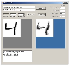 [Click on image for larger view.] Figure 3: Creating synthetic MNIST data.
The research experiments also showed that if you have a model trained using one dataset, then to train a second model using a similar dataset, if you start with the first model's trained weights and biases, the resulting second model is better than if had you started training from scratch. And the closer the two datasets are, the greater the increase in model accuracy.